Examples¶

Loading a Dataset and Exporting an Image ¶

This example loads a Plot3D dataset from fv.home/examples/f18 and exports an image.

import os

import fieldview as fv


# Resolve the bundled example dataset under the FieldView install root.
data_dir = os.path.join(fv.home, "examples", "f18")

# Load Plot3D (grid + results).
ds = fv.data.load_plot3d(
    os.path.join(data_dir, "f18i9b_g_bin"),
    os.path.join(data_dir, "f18i9b_q_bin"),
)

# Simple query and export.
print("Grids:", ds.num_grids)
output_png = os.path.join(os.path.expanduser("~"), "fv_plot3d.png")
fv.export_png(output_png)
print(f"Saved image: {output_png}")

Expected visual result:

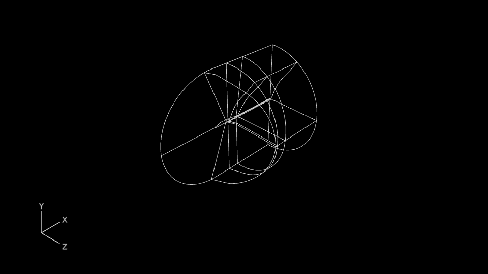
Expected result for load_export_example.py — Expected output from `load_export_example.py`.¶

Related API symbols:

Coordinate Surface ¶

This example creates 20 coordinate surfaces spaced across the X axis, applies scalar coloring with constant shading, disables outlines, and sets each surface transparency to 0.75.

import os

import fieldview as fv


data_dir = os.path.join(fv.home, "examples", "f18")

ds = fv.data.load_plot3d(
    os.path.join(data_dir, "f18i9b_g_bin"),
    os.path.join(data_dir, "f18i9b_q_bin"),
)

x_min = ds.xmin
x_max = ds.xmax
step = (x_max - x_min) / 19.0 if x_max != x_min else 0.0

fv.view.set_outline(False)

for i in range(20):
    cs = fv.vis.create_coord(
        ds,
        plane=fv.constant.Plane.X,
        x_plane=fv.RangedValue(value=x_min + i * step),
        transparency=0.75,
    )
    cs.coloring = fv.constant.Coloring.SCALAR
    cs.scalar_func = ds.scalar_functions[0]
    cs.display_type = fv.constant.DisplayType.CONSTANT

Expected visual result:

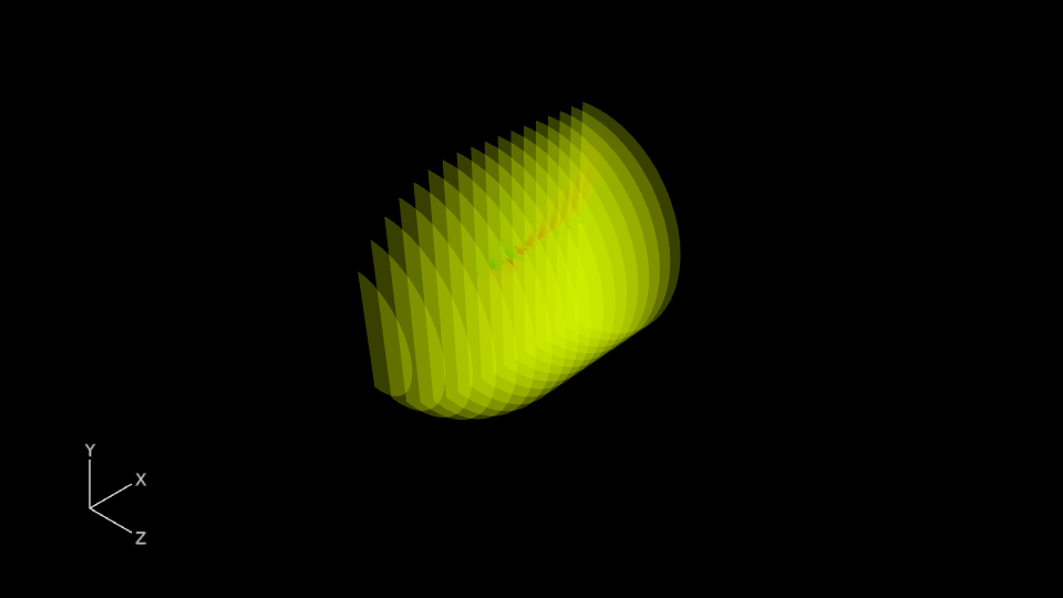
Expected result for coord_surface_example.py — Expected output from `coord_surface_example.py`.¶

Related API symbols:

Note

When modify(…) is available, PyFieldView can batch several property updates into one host-side modify command. For example, one round trip can update several coordinate-surface properties together:

cs.modify(
    coloring=fv.constant.Coloring.SCALAR,
    scalar_func=ds.scalar_functions[0],
    display_type=fv.constant.DisplayType.CONSTANT,
)

instead of separate round trips for:

cs.coloring = fv.constant.Coloring.SCALAR
cs.scalar_func = ds.scalar_functions[0]
cs.display_type = fv.constant.DisplayType.CONSTANT

If those values are known when the object is created and are not going to be modified later, prefer passing them directly to create_coord(…) so the surface is configured in the initial create call.

Computational Surface ¶

This example creates a computational surface on grid 1 and positions it along the I plane.

import os

import fieldview as fv


data_dir = os.path.join(fv.home, "examples", "f18")

ds = fv.data.load_plot3d(
    os.path.join(data_dir, "f18i9b_g_bin"),
    os.path.join(data_dir, "f18i9b_q_bin"),
)

cs = fv.vis.create_comp(ds, grid=1, plane=fv.constant.Plane.I)
cs.i_plane.value = 10
cs.coloring = fv.constant.Coloring.SCALAR
cs.colormap.name = fv.constant.ColormapName.SPECTRUM

Expected visual result:

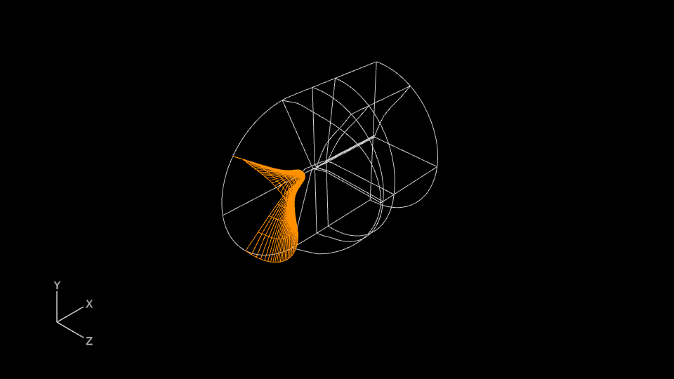
Expected result for comp_surface_example.py — Expected output from `comp_surface_example.py`.¶

Related API symbols:

Iso Surface ¶

This example creates an iso surface from "Mach number [PLOT3D]", sets its iso value to 0.31, applies scalar coloring and transparency, then adjusts the camera with zoom() and pan().

import os

import fieldview as fv


data_dir = os.path.join(fv.home, "examples", "f18")

ds = fv.data.load_plot3d(
    os.path.join(data_dir, "f18i9b_g_bin"),
    os.path.join(data_dir, "f18i9b_q_bin"),
)

fv.view.reset()

bnd = fv.vis.create_boundary(
    ds,
    types=fv.constant.BoundaryTypeSelection.ALL,
    display_type=fv.constant.DisplayType.SMOOTH,
)

iso_func_name = "Mach number [PLOT3D]"
iso = fv.vis.create_iso(ds, iso_func=iso_func_name)
iso.iso_value.value = 0.31
iso.coloring = fv.constant.Coloring.SCALAR
iso.display_type = fv.constant.DisplayType.SMOOTH
iso.transparency = 0.5

fv.camera.zoom(4.0)
fv.camera.pan(0.0, -0.05)

Expected visual result:

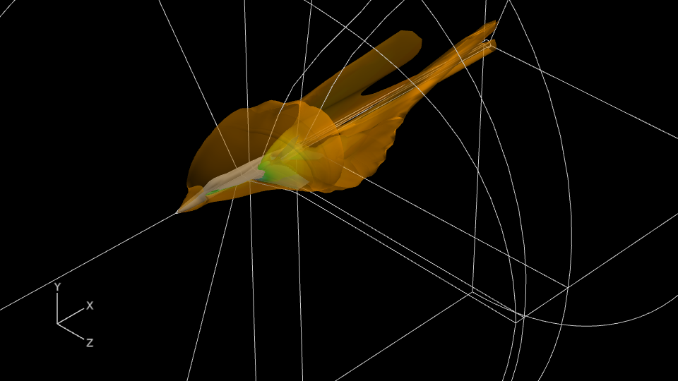
Expected result for iso_surface_example.py — Expected output from `iso_surface_example.py`.¶

Related API symbols:

Boundary Surface ¶

This example creates a boundary surface, enables all boundary types, and applies scalar coloring with a colormap.

import os

import fieldview as fv


data_dir = os.path.join(fv.home, "examples", "f18")

ds = fv.data.load_plot3d(
    os.path.join(data_dir, "f18i9b_g_bin"),
    os.path.join(data_dir, "f18i9b_q_bin"),
)

fv.view.reset()

bnd = fv.vis.create_boundary(ds, types=fv.constant.BoundaryTypeSelection.ALL)
bnd.coloring = fv.constant.Coloring.SCALAR
bnd.scalar_func = ds.scalar_functions[0]
bnd.display_type = fv.constant.DisplayType.MESH
bnd.colormap.name = fv.constant.ColormapName.SPECTRUM

fv.camera.zoom(16.0)
fv.camera.pan(0.06, -0.065)

Expected visual result:

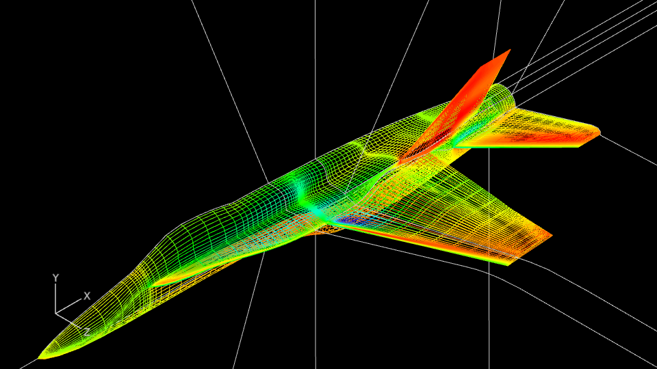
Expected result for boundary_surface_example.py — Expected output from `boundary_surface_example.py`.¶

Related API symbols:

Formula Creation ¶

This example loads the same Plot3D dataset twice, then creates formulas from both raw FieldView text and Python builder helpers. It also shows a dataset-comparison formula built with dataset_quantity(...).

import os

import fieldview as fv


data_dir = os.path.join(fv.home, "examples", "f18")

ds1 = fv.data.load_plot3d(
    os.path.join(data_dir, "f18i9b_g_bin"),
    os.path.join(data_dir, "f18i9b_q_bin"),
)

ds2 = fv.data.load_plot3d(
    os.path.join(data_dir, "f18i9b_g_bin"),
    os.path.join(data_dir, "f18i9b_q_bin"),
    input_mode=fv.constant.InputMode.APPEND,
)

qcrit = fv.formula.create(
    "Qcrit",
    'Qcriterion("Velocity Vectors [PLOT3D]")',
)

vel_mag = fv.formula.create(
    "Velocity Magnitude",
    fv.formula.mag("Velocity Vectors [PLOT3D]"),
)

delta_p = fv.formula.create(
    "Delta Pressure",
    fv.formula.dataset_quantity(2, "Pressure [PLOT3D]")
    - fv.formula.dataset_quantity(1, "Pressure [PLOT3D]"),
)

Related API symbols:

Exit FieldView ¶

This example exits the FieldView host directly from Python. Use fv.exit(status=...) when the intent is to terminate the application and report a specific result to a test harness, rather than passing "exit" through fieldview.fv_script().

import fieldview as fv


print("Exiting FieldView from Python with status 0.")
fv.exit(0)

Related API symbols:

Appending Datasets ¶

This example appends a second Plot3D dataset using the local-parallel configuration, then applies duplication and transform operations.

import os

import fieldview as fv


data_dir = os.path.join(fv.home, "examples", "f18")

# First load (replace).
ds0 = fv.data.load_plot3d(
    os.path.join(data_dir, "f18i9b_g_bin"),
    os.path.join(data_dir, "f18i9b_q_bin"),
)

# Second load (append) using local-parallel.
ds1 = fv.data.load_plot3d(
    os.path.join(data_dir, "f18i9b_g_bin"),
    os.path.join(data_dir, "f18i9b_q_bin"),
    input_mode=fv.constant.InputMode.APPEND,
    server_config=fv.constant.ServerConfig.LOCAL_PARALLEL,
)

# Mirror and translate the appended dataset (apply immediately).
ds1.duplication.mirror.axes = fv.constant.Axes.Z
ds1.transform.translate = (0.0, 0.0, 15.0)

print("Grids:", ds0.num_grids, ds1.num_grids)

fv.view.reset()
fv.camera.zoom(2.0)

Expected visual result:

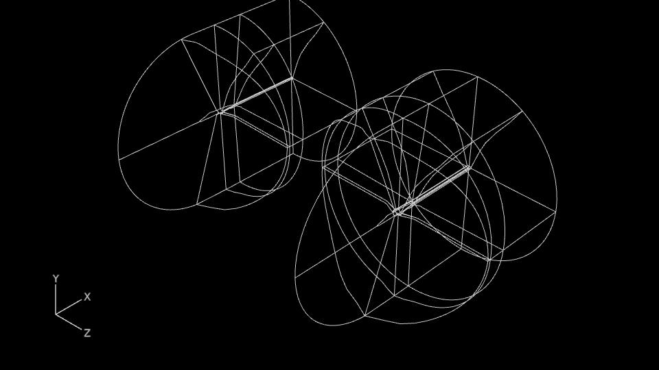
Expected result for load_append_example.py — Expected output from `load_append_example.py`.¶

Related API symbols:

Point Probes ¶

This example probes the current scalar and vector functions at a displayed point and at a structured-grid IJK location.

import os

import fieldview as fv


data_dir = os.path.join(fv.home, "examples", "f18")

ds = fv.data.load_plot3d(
    os.path.join(data_dir, "f18i9b_g_bin"),
    os.path.join(data_dir, "f18i9b_q_bin"),
)

display_probe = fv.data.probe((0.01, 0.02, 0.01), dataset=ds)
ijk_probe = fv.data.probe_ijk((2, 3, 4), grid=1, dataset=ds)

print("Display probe scalar:", display_probe.scalar)
print("IJK probe point:", ijk_probe.point)

Related API symbols:

Integration ¶

This example creates a boundary surface and a coordinate surface, integrates a scalar over the boundary selection, then integrates over a connected partial region on the coordinate surface. It also writes a summary of those results into a screen annotation.

import os
from typing import Optional

import fieldview as fv


data_dir = os.path.join(fv.home, "examples", "f18")

ds = fv.data.load_plot3d(
    os.path.join(data_dir, "f18i9b_g_bin"),
    os.path.join(data_dir, "f18i9b_q_bin"),
)

fv.view.reset()

scalar_name = ds.scalar_functions[0]
probe = fv.data.probe_ijk((2, 3, 4), grid=1, dataset=ds)

boundary = fv.vis.create_boundary(ds, types=fv.constant.BoundaryTypeSelection.ALL)
boundary.scalar_func = scalar_name

coord = fv.vis.create_coord(ds)
coord.scalar_func = scalar_name
coord.plane = fv.constant.Plane.X
coord.x_plane.value = probe.point.x

boundary_result = boundary.integrate()
coord_partial_result = coord.integrate_partial_surface(tuple(probe.point))

print(boundary_result)
print(coord_partial_result)


def _integration_summary(
    label: str, result: Optional[fv.data.IntegrationResult]
) -> str:
    if result is None:
        return f"{label}: no result"
    average = "n/a" if result.average is None else f"{result.average:.6g}"
    return f"{label}: sum={result.sum:.6g}, area={result.area:.6g}, avg={average}"


fv.vis.create_annotation_text(
    "\n".join(
        [
            _integration_summary("Boundary", boundary_result),
            _integration_summary("Coord partial", coord_partial_result),
        ]
    ),
    position=(20, 80),
    color=fv.constant.GeometricColor.WHITE,
    font_size=18,
)

fv.camera.pan(0.25, -0.1)

Expected visual result:

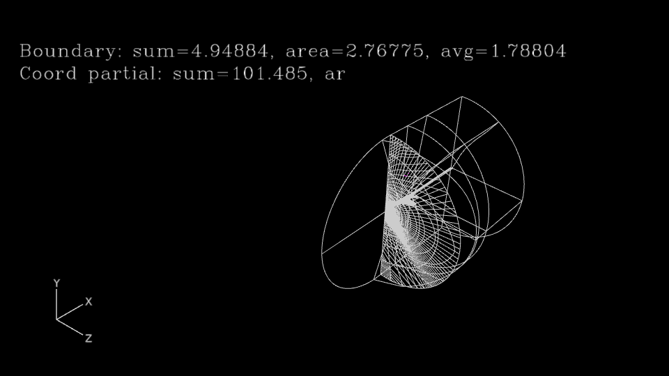
Expected result for integration_example.py — Expected output from `integration_example.py`.¶

Related API symbols:

Streamlines ¶

This example creates streamlines, adds seeds, and calculates the paths.

import os

import fieldview as fv


data_dir = os.path.join(fv.home, "examples", "f18")

ds = fv.data.load_plot3d(
    os.path.join(data_dir, "f18i9b_g_bin"),
    os.path.join(data_dir, "f18i9b_q_bin"),
)

fv.view.set_outline(True)
fv.view.reset()

bnd = fv.vis.create_boundary(
    ds,
    types=fv.constant.BoundaryTypeSelection.ALL,
    display_type=fv.constant.DisplayType.SMOOTH,
)

sl = fv.vis.create_streamlines(
    ds,
    vector_func="Velocity Vectors [PLOT3D]",
    coloring=fv.constant.Coloring.SCALAR,
    scalar_func=ds.scalar_functions[0],
    display_type=fv.constant.PathsDisplayType.RIBBONS,
    seed_coord=fv.constant.StreamlinesSeedCoord.XYZ,
    ribbon_width=4,
)

start = (0.25, 0.0, 0.25)
end = (1.5, 0.0, 0.25)
num_seeds = 10

seeds = [
    (
        start[0] + (end[0] - start[0]) * i / (num_seeds - 1),
        start[1] + (end[1] - start[1]) * i / (num_seeds - 1),
        start[2] + (end[2] - start[2]) * i / (num_seeds - 1),
    )
    for i in range(num_seeds)
]

sl.add_seeds(seeds)
sl.calculate()

fv.camera.zoom(6.0)
fv.camera.pan(0.0, -0.075)

Expected visual result:

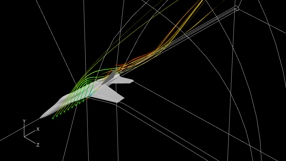
Expected result for streamlines_example.py — Expected output from `streamlines_example.py`.¶

Changing sl.seed_coord after seeds have been added is rejected. Call sl.delete_all_seeds() first if you need to switch between IJK, IJK_REAL, and XYZ seed coordinates.

When using sl.seed_surface(...), the source surface must still be live and must come from the same dataset as the streamline object.

Streak controls follow one Python-side contract: release_interval must be greater than 0 and duration must be greater than 0 and smaller than release_interval. Invalid values are rejected before any core call.

Related API symbols:

Particle Paths ¶

This example imports a particle-path file, applies scalar coloring, and enables animation.

import os

import fieldview as fv


data_dir = os.path.join(fv.home, "examples", "f18")

ds = fv.data.load_plot3d(
    os.path.join(data_dir, "f18i9b_g_bin"),
    os.path.join(data_dir, "f18i9b_q_bin"),
)

ppath_file = os.path.join(os.path.dirname(__file__), "particle_paths_example.fvp")

ppath = fv.vis.create_particle_paths(
    ds,
    filename=ppath_file,
    coloring=fv.constant.Coloring.SCALAR,
    scalar_func="Duration",
    display_type=fv.constant.PathsDisplayType.SPHERES_AND_LINES,
    animate=True,
    animate_direction=fv.constant.AnimationDirection.FORWARD,
    animate_divs=25,
)

ppath.select_by_initial_value = True
ppath.select_by_initial_value_variable = "Duration"

Related API symbols:

2D Plot ¶

This example creates a 2D plot on the current dataset, defines one centerline volume path, and exports that path using FieldView’s native path text format. Non-fatal Plot2D host diagnostics are emitted as Python warnings and may appear in the Python console during interactive use.

import os

import fieldview as fv


data_dir = os.path.join(fv.home, "examples", "f18")
ds = fv.data.load_plot3d(
    os.path.join(data_dir, "f18i9b_g_bin"),
    os.path.join(data_dir, "f18i9b_q_bin"),
)
left_func = ds.scalar_functions[0]
mid_y = 0.5 * (ds.ymin + ds.ymax)
mid_z = 0.5 * (ds.zmin + ds.zmax)
start = (ds.xmin + 0.2 * (ds.xmax - ds.xmin), mid_y, mid_z)
end = (ds.xmin + 0.4 * (ds.xmax - ds.xmin), mid_y, mid_z)

plot = fv.vis.create_plot2d(
    left_axis_func=left_func,
    show_plot=True,
    show_path=True,
)

path = plot.create_line_path_volume(
    start,
    end,
)

plot.left_axis.label = left_func
plot.horizontal_axis.label = "Distance"
output_txt = os.path.join(os.path.expanduser("~"), "line_path.txt")
path.export_txt(output_txt)
print(f"Saved path data: {output_txt}")

Expected visual result:

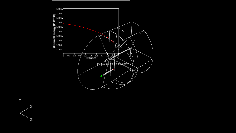
Expected result for plot2d_example.py — Expected output from `plot2d_example.py`.¶

Related API symbols:

Surface Flows ¶

This example creates a surface flow object, updates its scalar path variable, calculates the flow, and enables a local colormap range.

import os

import fieldview as fv


data_dir = os.path.join(fv.home, "examples", "f18")

ds = fv.data.load_plot3d(
    os.path.join(data_dir, "f18i9b_g_bin"),
    os.path.join(data_dir, "f18i9b_q_bin"),
)

fv.view.reset()

bnd = fv.vis.create_boundary(
    ds,
    types=fv.constant.BoundaryTypeSelection.ALL,
    display_type=fv.constant.DisplayType.SMOOTH,
)

sf = fv.vis.create_surface_flows(
    ds,
    mode=fv.constant.SurfaceFlowMode.EULER,
    vector_func="Velocity Vectors [PLOT3D]",
    coloring=fv.constant.Coloring.SCALAR,
    scalar_path_variable=ds.scalar_functions[0],
    direction=fv.constant.CalculationDirection.BOTH,
    seeding=fv.constant.SurfaceFlowSeeding.MEDIUM_DENSITY,
    step=21,
)
sf.scalar_path_variable = "Speed of sound [PLOT3D]"
sf.calculate()

sf.colormap.use_local = True

fv.camera.zoom(16.0)
fv.camera.pan(0.06, -0.065)

Expected visual result:

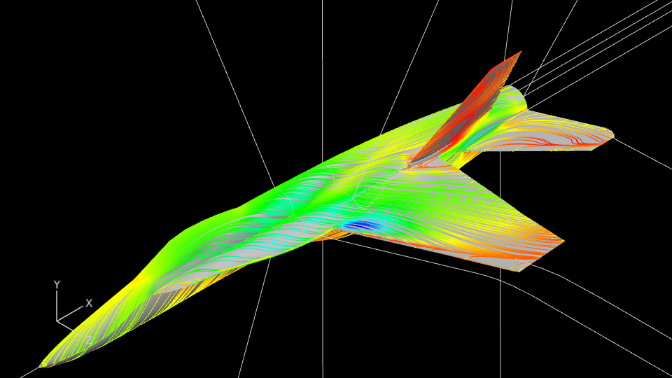
Expected result for surface_flows_example.py — Expected output from `surface_flows_example.py`.¶

Related API symbols:

Vortex Cores ¶

This example creates a vortex-cores surface, enables scalar coloring, and sets the scalar colormap.

import os

import fieldview as fv


data_dir = os.path.join(fv.home, "examples", "f18")

ds = fv.data.load_plot3d(
    os.path.join(data_dir, "f18i9b_g_bin"),
    os.path.join(data_dir, "f18i9b_q_bin"),
)

vc = fv.vis.create_vortex_cores(
    ds,
    method=fv.constant.VortexCoreMethod.VORTICITY_ALIGNMENT,
    vector_func=ds.vector_functions[0],
)
vc.coloring = fv.constant.Coloring.SCALAR
vc.scalar_path_variable = "Vortex Strength"
vc.colormap.name = fv.constant.ColormapName.SPECTRUM

Expected visual result:

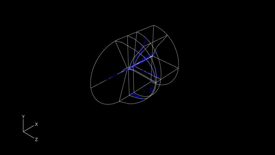
Expected result for vortex_cores_example.py — Expected output from `vortex_cores_example.py`.¶

Related API symbols:

fieldview.vis.create_vortex_cores()
fieldview.vis.VortexCores
fieldview.vis.VortexCores.coloring
fieldview.vis.VortexCores.scalar_path_variable
fieldview.vis.VortexCores.colormap

Transient ¶

This example loads a transient FV-UNS dataset and inspects metadata, then selects a time step and runs a simple transient sweep.

Dataset.sweep_time() supports four explicit range modes:

time-step values via from_time_step / to_time_step
time-step indices via from_time_step_index / to_time_step_index
solution-time values via from_solution_time / to_solution_time
solution-time indices via from_solution_time_index / to_solution_time_index

Calling ds.sweep_time() with no range arguments defaults to from_time_step_index=0 and to_time_step_index=-1.

import os

import fieldview as fv


uns_file = os.path.join(fv.home, "examples", "rectangular_duct", "rect_duct_010.uns")

# Load the dataset in transient mode.
ds = fv.data.load_fvuns(uns_file, transient=True)

# Query the available time-step and solution-time values.
info = ds.transient_info()
print("Current step:", info.time_step)
print("First three steps:", info.time_step_values[:3])

# Select a specific time step for inspection.
ds.set_transient(time_step=25)

cs = fv.vis.create_coord(
    ds,
    plane=fv.constant.Plane.Z,
    coloring=fv.constant.Coloring.SCALAR,
    display_type=fv.constant.DisplayType.CONSTANT,
)

# Sweep all transient time steps (default: step indices 0 to -1).
ds.sweep_time()

Related API symbols:

Registry Arrays + Derived Functions ¶

This example reads scalar, vector, and native XYZ position snapshots, then creates derived scalar and vector functions from NumPy arrays.

import os

import numpy as np

import fieldview as fv


data_dir = os.path.join(fv.home, "examples", "f18")
ds = fv.data.load_plot3d(
    os.path.join(data_dir, "f18i9b_g_bin"),
    os.path.join(data_dir, "f18i9b_q_bin"),
)

scalar_name = ds.scalar_functions[0]
vector_name = ds.vector_functions[0]
distance_field_name = "Distance From Point"
vector_to_point_field_name = "Vector To Point"

# Show array-view behavior on the first grid.
pressure = ds.scalars.to_numpy(scalar_name, grid=1, copy=False)
velocity = ds.vectors.to_numpy(vector_name, grid=1, copy=False)
xyz = ds.positions.to_numpy(grid=1, copy=False)

# copy=False returns read-only NumPy views when possible.
# The returned arrays keep the snapshot backing alive, so they remain valid
# even after the local ``snap`` variable is gone.
print("pressure writeable:", pressure.flags.writeable)
print("velocity shape:", velocity.shape)
print("xyz shape:", xyz.shape)

ref_point = np.array([2.0, 1.0, 0.05], dtype=float)

# Create/update registry arrays on every dataset grid.
for grid in range(1, ds.num_grids + 1):
    xyz_grid = ds.positions.to_numpy(grid=grid, copy=False)
    vector_to_point = ref_point - np.array(xyz_grid, copy=True)
    distance = np.linalg.norm(vector_to_point, axis=1)

    ds.scalars.create(distance_field_name, distance, grid=grid)
    ds.vectors.create(vector_to_point_field_name, vector_to_point, grid=grid)

# Create a Z-plane coordinate surface and color it by the distance field.
coord = fv.vis.create_coord(
    ds,
    plane=fv.constant.Plane.Z,
    z_plane=fv.RangedValue(value=0.05),
    coloring=fv.constant.Coloring.SCALAR,
    scalar_func=distance_field_name,
    vector_func=vector_to_point_field_name,
    display_type=fv.constant.DisplayType.CONSTANT,
)

# Create a second Z-plane coord surface with vector display.
coord_vectors = fv.vis.create_coord(
    ds,
    plane=fv.constant.Plane.Z,
    z_plane=fv.RangedValue(value=0.05),
    coloring=fv.constant.Coloring.GEOMETRIC,
    geometric_color=fv.constant.GeometricColor.WHITE,
    vector_func=vector_to_point_field_name,
    display_type=fv.constant.DisplayType.VECTORS,
    vector_options=fv.VectorOptions(vector_scale=2.0),
)

Expected visual result:

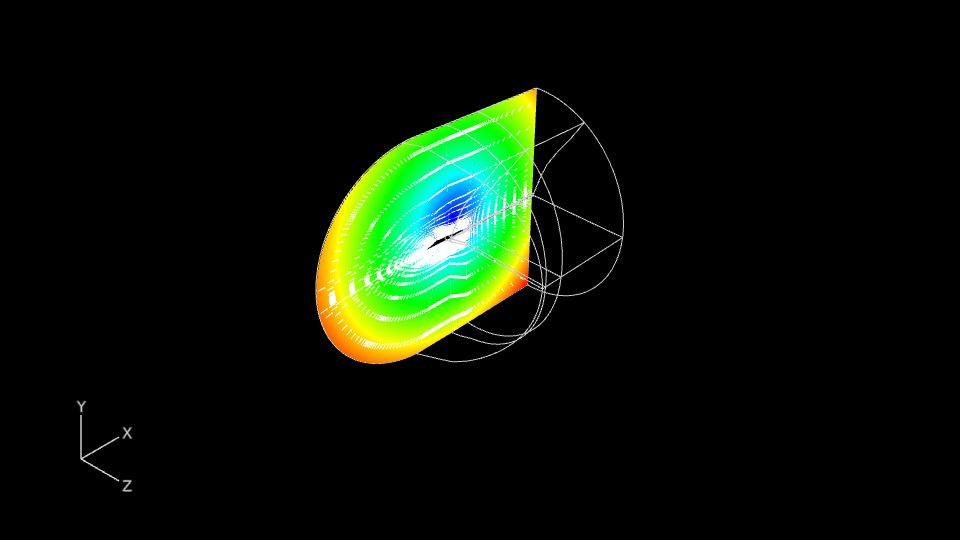
Expected result for registry_arrays_example.py — Expected output from `registry_arrays_example.py`.¶

Related API symbols:

Transient datasets ¶

For transient datasets, fieldview.data.ScalarRegistry.create() and fieldview.data.VectorRegistry.create() write values for the currently active time step (the one selected with ds.set_transient(...)).

To define custom arrays for multiple time steps, loop over time steps and call create(...) after selecting each step.

for step in ds.transient_info().time_step_values:
    ds.set_transient(time_step=step)
    values = compute_values_for_step(ds)
    ds.scalars.create("My Scalar", values, grid=1)

Behavior when not all time steps are explicitly written:

If you write a custom scalar/vector at only one time step, that same data is reused for all time steps.
If you write data at some time steps only, FieldView reuses the most recent previous stored frame for intermediate steps.
For steps before the first stored frame, the first stored frame is used.
For steps after the last stored frame, the last stored frame is used.
No interpolation is applied between stored time steps.

Accessing Scene Objects ¶

PyFieldView can access and modify objects that were already created before the current PyFieldView script started.

Create scene content ¶

Run this once to load a dataset and create a boundary surface that the next script can discover and modify.

import os

import fieldview as fv


# Prep script: load data and create one boundary surface in the scene.
data_dir = os.path.join(fv.home, "examples", "f18")
ds = fv.data.load_plot3d(
    os.path.join(data_dir, "f18i9b_g_bin"),
    os.path.join(data_dir, "f18i9b_q_bin"),
)

bnd = fv.vis.create_boundary(ds, types=fv.constant.BoundaryTypeSelection.ALL)


print("Prepared with one boundary surface.")

Discover and update objects ¶

This script uses fv.data.get_session_state() and fv.get_all_objects() to fetch existing objects, grab the first boundary surface, then:

reset the current view
turn off grid/outline display
set display type to smooth
show scalar min/max
show mesh

import fieldview as fv


# get_session_state(): one-shot session snapshot (data loaded flag, bounds,
# function lists, and grouped object info) useful for startup checks.
state = fv.data.get_session_state()
if not state.data_loaded:
    raise RuntimeError("No dataset is loaded. Run the prep script first.")

# get_all_objects(): returns live typed wrappers you can modify directly
# (Boundary/Coord/Comp/Iso/Paths/etc.) in the current session.
objects = fv.get_all_objects()
if not objects.boundary_list:
    raise RuntimeError("No boundary surface found. Run the prep script first.")

bnd = objects.boundary_list[0]

# Requested edits on the existing boundary/view.
fv.view.set_outline(False)  # turn off outline/grid view
bnd.coloring = fv.constant.Coloring.SCALAR
bnd.display_type = fv.constant.DisplayType.SMOOTH
bnd.scalar_minmax.show = True
bnd.show_mesh = True

fv.view.reset()
fv.camera.zoom(3.0)
fv.camera.pan(0.06, 0.0)

print("Reused boundary object and updated display settings.")

Expected visual result:

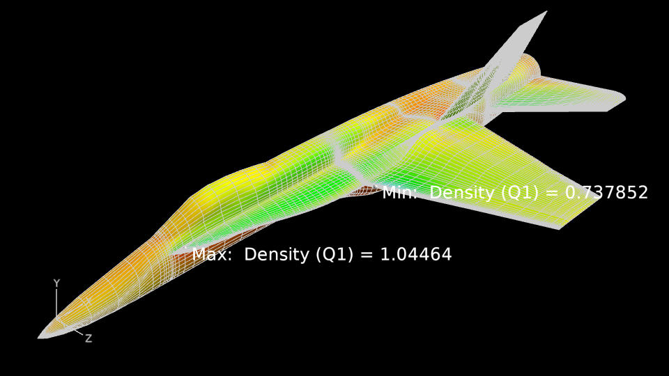
Expected result for scene_objects_reuse_boundary_example.py — Expected output from `scene_objects_reuse_boundary_example.py`.¶

Related API symbols:

Layout Management + View Control ¶

This example uses the public fieldview.layout and fieldview.view submodules to split one window into two panes and apply a different view in the second pane. View functions default to the current window and also accept window= for direct targeting. The same API works in interactive and batch graphics sessions.

When examples are run back-to-back in the same FV session, remember that view display toggles such as outline are shared session state. Because reset(), center(), and fit() all depend on the currently visible scene contents, running another script after changing them can affect how reset(), center(), or fit() frame the scene. Set outline explicitly when an example depends on it.

For deterministic scripted navigation, call fieldview.view.reset() before a sequence of fieldview.view or fieldview.camera operations. This resets the world/view transform, but view display toggles such as outline must still be set explicitly if your script depends on them.

A good default sequence after loading a dataset is:

set view display toggles such as outline explicitly
call fieldview.view.reset()
create any view-size-dependent objects
apply final fieldview.camera adjustments at the end

This helps keep scripted results reproducible because some invariant-size or screen-sized objects can depend on the current view state at creation time.

reset(), center(), and fit() are related but not equivalent:

fieldview.view.reset() performs the UI reset action for the world transform. It recenters the visible scene and restores the default view orientation.
fieldview.view.center() recenters the visible scene, or centers a specific world-space point when x, y, and z are provided. It preserves the current viewing orientation.
fieldview.view.fit() adjusts the current view so the visible scene fits well in the window while preserving the current viewing orientation.

import os

import fieldview as fv


data_dir = os.path.join(fv.home, "examples", "f18")

ds = fv.data.load_plot3d(
    os.path.join(data_dir, "f18i9b_g_bin"),
    os.path.join(data_dir, "f18i9b_q_bin"),
)

split = fv.layout.split_horizontal(mode="copy", window=1)

# Keep windows independent; otherwise view changes in one pane can affect both.
fv.layout.set_view_sync(False, window=1)
fv.layout.set_view_sync(False, window=split.new_window)

fv.view.reset(window=1)
fv.view.set_perspective(False, window=1)
fv.view.align("+y", window=1)

fv.view.reset(window=split.new_window)
fv.view.set_perspective(False, window=split.new_window)
fv.view.align("+x", window=split.new_window)

Expected visual result:

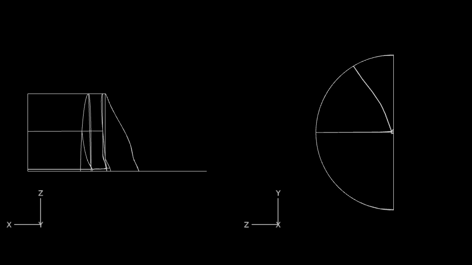
Expected result for window_view_example.py — Expected output from `window_view_example.py`.¶

Related API symbols:

Camera Navigation ¶

This example uses the public fieldview.camera submodule for direct scripted navigation and deterministic camera state capture. It demonstrates look_at() to define a reproducible camera pose, then uses get_pose() to inspect the resulting eye/target/up values. It then performs an orbit sequence in a single window and shows get_state() before and after the scripted motion.

Note: get_pose() is intended for inspection and pose-style workflows with look_at(). For exact view replay, prefer get_state() + set_state().

import os

import fieldview as fv

# Load sample PLOT3D dataset bundled with FieldView.
data_dir = os.path.join(fv.home, "examples", "f18")
ds = fv.data.load_plot3d(
    os.path.join(data_dir, "f18i9b_g_bin"),
    os.path.join(data_dir, "f18i9b_q_bin"),
)
# Add a boundary surface so camera motion is visible.
fv.vis.create_boundary(
    ds,
    types=fv.constant.BoundaryTypeSelection.ALL,
    display_type=fv.constant.DisplayType.SMOOTH,
)

print(f"Loaded dataset_id={ds.dataset_id}")

fv.view.reset()
fv.view.set_perspective(True, angle=25.0)

# Capture deterministic state before scripted camera motion.
# Use get_state()/set_state() for exact replay across sessions.
baseline_state = fv.camera.get_state()
print("Deterministic view state:", baseline_state)

# Set a reproducible starting camera pose.
fv.camera.look_at(
    eye=(-1.0, 0.0, 0.0),
    target=(0.0, 0.0, 0.0),
    up=(0.0, 1.0, 0.0),
)

# Inspect pose after look_at().
# Use get_pose() for pose-style workflows (eye/target/up).
pose = fv.camera.get_pose()
print("Pose after look_at:", pose)

# Run the orbit sequence.
for _ in range(90):
    fv.camera.orbit(1.0, 0.0)

for _ in range(90):
    fv.camera.orbit(-1.0, 0.0)

for _ in range(90):
    fv.camera.orbit(0.0, 1.0)

for _ in range(90):
    fv.camera.orbit(0.0, -1.0)

# Log final pose and deterministic state after scripted motion.
print("Final pose:", fv.camera.get_pose())
print("Final deterministic view state:", fv.camera.get_state())

Related API symbols:

Examples¶

Loading a Dataset and Exporting an Image ¶

Coordinate Surface ¶

Computational Surface ¶

Iso Surface ¶

Boundary Surface ¶

Formula Creation ¶

Exit FieldView ¶

Appending Datasets ¶

Point Probes ¶

Integration ¶

Streamlines ¶

Particle Paths ¶

2D Plot ¶

Surface Flows ¶

Vortex Cores ¶

Transient ¶

Registry Arrays + Derived Functions ¶

Transient datasets ¶

Accessing Scene Objects ¶

Create scene content ¶

Discover and update objects ¶

Layout Management + View Control ¶

Camera Navigation ¶

Table of Contents

This Page